BatchNorm原理

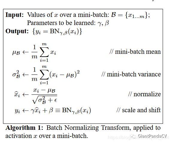
这是论文中给出的对BatchNorm的算法流程解释,这篇推文的目的主要是推导和从源码角度解读BatchNorm的前向传播和反向传播,就不关注具体的原理了(实际上是因为BN层的原理非常复杂),我们暂时知道BN层是用来调整数据分布,降低过拟合的就够了。

前向传播推导

前向传播实际就是将Algorithm1的4个公式转化为编程语言,这里先贴一段CS231N官方提供的代码:

1
2
3
4
5
6
7
8
9
10
11
12
13
14
15
16
17
18
19
20
21
22
23
24
25
26
27
28
29
30
31
32
33
34
35
36
37
38
39
40
41
42
43
44
45
46
47
def batchnorm_forward(x, gamma, beta, bn_param):
"""
Input:
- x: (N, D)维输入数据
- gamma: (D,)维尺度变化参数
- beta: (D,)维尺度变化参数
- bn_param: Dictionary with the following keys:
- mode: 'train' 或者 'test'
- eps: 一般取1e-8~1e-4
- momentum: 计算均值、方差的更新参数
- running_mean: (D,)动态变化array存储训练集的均值
- running_var:(D,)动态变化array存储训练集的方差

Returns a tuple of:
- out: 输出y_i(N,D)维
- cache: 存储反向传播所需数据
"""
mode = bn_param['mode']
eps = bn_param.get('eps', 1e-5)
momentum = bn_param.get('momentum', 0.9)

N, D = x.shape
# 动态变量,存储训练集的均值方差
running_mean = bn_param.get('running_mean', np.zeros(D, dtype=x.dtype))
running_var = bn_param.get('running_var', np.zeros(D, dtype=x.dtype))

out, cache = None, None
# TRAIN 对每个batch操作
if mode == 'train':
sample_mean = np.mean(x, axis = 0)
sample_var = np.var(x, axis = 0)
x_hat = (x - sample_mean) / np.sqrt(sample_var + eps)
out = gamma * x_hat + beta
cache = (x, gamma, beta, x_hat, sample_mean, sample_var, eps)
running_mean = momentum * running_mean + (1 - momentum) * sample_mean
running_var = momentum * running_var + (1 - momentum) * sample_var
# TEST:要用整个训练集的均值、方差
elif mode == 'test':
x_hat = (x - running_mean) / np.sqrt(running_var + eps)
out = gamma * x_hat + beta
else:
raise ValueError('Invalid forward batchnorm mode "%s"' % mode)

bn_param['running_mean'] = running_mean
bn_param['running_var'] = running_var

return out, cache

就是一个公式带入的问题,这里倒是没啥好说的,不过了为了和下面反向传播对比理解,这里我们明确每一个张量的维度:

  • x shape为(N,D),可以将N看成batch size,D看成特征图展开为1列的元素个数
  • gamma shape为(D,)
  • beta shape为(D,)
  • running_mean shape为(D,)
  • running_var shape为(D,)

请特别注意滑动平均(影子变量)这种Trick的引入,目的是为了控制变量更新的速度,防止变量的突然变化对变量的整体影响,这能提高模型的鲁棒性。

反向传播推导

这才是重点,现在做一些约定:

  • $\delta$为一个Batch所有样本的方差
  • $\mu$为样本均值
  • $\hat{x}$为归一化后的样本数据
  • $y_{i}$为输入样本$x_{i}$经过尺度变化的输出量
  • $\gamma$和$\beta$为尺度变化系数
  • $\frac{\partial L}{\partial y}$是上一层的梯度,并假设$x$和$y$都是$(\mathrm{N}, \mathrm{D})$维,即有N个维度为D的样本在BN层的前向传播中$x_{i}$通过$\gamma, \beta, \hat{x}$将$x_{i}$变换为$y_{i}$,那么反向传播则是根据$\frac{\partial L}{\partial y_{i}}$求得$\frac{\partial L}{\partial \gamma}, \frac{\partial L}{\partial \beta}, \frac{\partial L}{\partial x_{i}}$
  • 求解$\frac{\partial L}{\partial \gamma}$ $\frac{\partial L}{\partial \gamma}=\sum_{i} \frac{\partial L}{\partial y_{i}} \frac{\partial y_{i}}{\partial \gamma}=\sum_{i} \frac{\partial L}{\partial y_{i}} \hat{x}$
  • 求解$\frac{\partial L}{\partial \beta}$ $\frac{\partial L}{\partial \beta}=\sum_{i} \frac{\partial L}{\partial y_{i}} \frac{\partial y_{i}}{\partial \beta}=\sum_{i} \frac{\partial L}{\partial y_{i}}$
  • 求解$\frac{\partial L}{\partial x_{i}}$根据论文的公式和链式法则可得下面的等式: $\frac{\partial L}{\partial x_{i}}=\frac{\partial L}{\partial \widehat{x}_{i}} \frac{\partial \widehat{x}_{i}}{\partial x_{i}}+\frac{\partial L}{\partial \sigma} \frac{\partial \sigma}{\partial x_{i}}+\frac{\partial L}{\partial \mu} \frac{\partial \mu}{\partial x_{i}}$我们这里又可以先求$\frac{\partial L}{\partial \hat{x}}$
  • $\frac{\partial L}{\partial \hat{x}}=\frac{\partial L}{\partial y} \frac{\partial y}{\partial \hat{x}}=\frac{\partial L}{\partial y} \gamma$ (1)
  • $\frac{\partial L}{\partial \sigma}=\sum_{i} \frac{\partial L}{\partial y_{i}} \frac{\partial y_{i}}{\partial \hat{x}_{i}} \frac{\partial \hat{x}_{i}}{\partial \sigma}=-\frac{1}{2} \sum_{i} \frac{\partial L}{\partial \widehat{x}_{i}}\left(x_{i}-\mu\right)(\sigma+\varepsilon)^{-1.5}$ (2)
  • $\frac{\partial L}{\partial \mu}=\frac{\partial L}{\partial \hat{x}} \frac{\partial \hat{x}}{\partial \mu}+\frac{\partial L}{\partial \sigma} \frac{\partial \sigma}{\partial \mu}=\sum_{i} \frac{\partial L}{\partial \hat{x}_{i}} \frac{-1}{\sqrt{\sigma+\varepsilon}}+\frac{\partial L}{\partial \sigma} \frac{-2 \Sigma_{i}\left(x_{i}-\mu\right)}{N}$ (3)
  • 有了(1) (2) (3)就可以求出$\frac{\partial L}{\partial x_{i}}$
    $\frac{\partial L}{\partial x_{i}}=\frac{\partial L}{\partial \widehat{x}_{i}} \frac{\partial \widehat{x}_{i}}{\partial x_{i}}+\frac{\partial L}{\partial \sigma} \frac{\partial \sigma}{\partial x_{i}}+\frac{\partial L}{\partial \mu} \frac{\partial \mu}{\partial x_{i}}=\frac{\partial L}{\partial \hat{x}_{i}} \frac{1}{\sqrt{\sigma+\varepsilon}}+\frac{\partial L}{\partial \sigma} \frac{2\left(x_{i}-\mu\right)}{N}+\frac{\partial L}{\partial \mu} \frac{1}{N}$

到这里就推到出了BN层的反向传播公式了,和论文中一样,截取一下论文中的结果图:
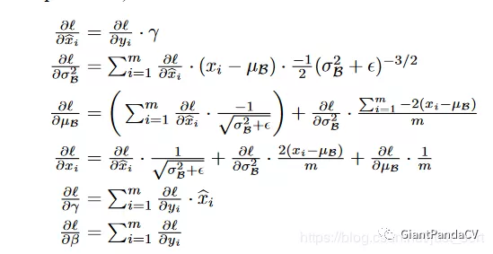
贴一份CS231N反向传播代码:

1
2
3
4
5
6
7
8
9
10
11
12
13
14
15
16
17
18
19
20
21
22
23
def batchnorm_backward(dout, cache):
"""
Inputs:
- dout: 上一层的梯度,维度(N, D),即 dL/dy
- cache: 所需的中间变量,来自于前向传播

Returns a tuple of:
- dx: (N, D)维的 dL/dx
- dgamma: (D,)维的dL/dgamma
- dbeta: (D,)维的dL/dbeta
"""
x, gamma, beta, x_hat, sample_mean, sample_var, eps = cache
N = x.shape[0]

dgamma = np.sum(dout * x_hat, axis = 0)
dbeta = np.sum(dout, axis = 0)

dx_hat = dout * gamma
dsigma = -0.5 * np.sum(dx_hat * (x - sample_mean), axis=0) * np.power(sample_var + eps, -1.5)
dmu = -np.sum(dx_hat / np.sqrt(sample_var + eps), axis=0) - 2 * dsigma*np.sum(x-sample_mean, axis=0)/ N
dx = dx_hat /np.sqrt(sample_var + eps) + 2.0 * dsigma * (x - sample_mean) / N + dmu / N

return dx, dgamma, dbeta

DarkNet代码详解

1. 构造BN层

构造BN层的代码在src/batchnorm_layer.c中实现,详细代码如下:

1
2
3
4
5
6
7
8
9
10
11
12
13
14
15
16
17
18
19
20
21
22
23
24
25
26
27
28
29
30
31
32
33
34
35
36
37
38
39
layer make_batchnorm_layer(int batch, int w, int h, int c, int train)
{
fprintf(stderr, "Batch Normalization Layer: %d x %d x %d image\n", w,h,c);
layer layer = { (LAYER_TYPE)0 };
layer.type = BATCHNORM; // 网络层的名字
layer.batch = batch; //一个batch中包含的图片数
layer.train = train;
layer.h = layer.out_h = h; // 当前层的输出高度等于输入高度h
layer.w = layer.out_w = w; // 当前层的输出宽度等于输入宽度w
layer.c = layer.out_c = c; // 当前层的输出通道数等于输入通道数

layer.n = layer.c;
layer.output = (float*)xcalloc(h * w * c * batch, sizeof(float)); // layer.output为该层所有的输出(包括mini-batch所有输入图片的输出)
layer.delta = (float*)xcalloc(h * w * c * batch, sizeof(float)); //layer.delta 是该层的敏感度图,和输出的维度想同
layer.inputs = w*h*c; //mini-batch中每张输入图片的像素元素个数
layer.outputs = layer.inputs; // 对应每张输入图片的所有输出特征图的总元素个数(每张输入图片会得到n也即layer.out_c张特征图)

layer.biases = (float*)xcalloc(c, sizeof(float)); // BN层特有参数,缩放系数
layer.bias_updates = (float*)xcalloc(c, sizeof(float)); // 缩放系数的敏感度图

layer.scales = (float*)xcalloc(c, sizeof(float)); // BN层特有参数,偏置系数
layer.scale_updates = (float*)xcalloc(c, sizeof(float)); // 偏置系数的敏感度图
int i;
for(i = 0; i < c; ++i){
layer.scales[i] = 1; // 将缩放系数初始化为1
}

layer.mean = (float*)xcalloc(c, sizeof(float)); // mean 一个batch中所有图片的均值,分通道求取
layer.variance = (float*)xcalloc(c, sizeof(float)); // variance 一个batch中所有图片的方差,分通道求取

layer.rolling_mean = (float*)xcalloc(c, sizeof(float)); // 均值的滑动平均,影子变量
layer.rolling_variance = (float*)xcalloc(c, sizeof(float)); // 方差的滑动平均,影子变量

layer.forward = forward_batchnorm_layer; // 前向传播函数
layer.backward = backward_batchnorm_layer; // 反向传播函数
layer.update = update_batchnorm_layer;
...
return layer;
}

2.前向传播公式实现

DarkNet中在src/blas.h中实现了前向传播的几个公式:

1
2
3
4
5
6
7
8
9
10
11
12
13
14
15
16
17
18
19
20
21
22
23
24
25
26
27
28
29
30
31
32
33
34
35
36
37
38
39
40
41
42
43
44
45
46
47
48
49
50
51
52
53
54
55
56
57
58
59
60
61
62
63
64
65
66
67
68
69
70
71
72
73
74
75
76
77
78
79
80
81
82
83
84
85
86
87
88
89
90
91
92
93
94
95
96
97
98
/*
** 计算输入数据x的平均值,输出的mean是一个矢量,比如如果x是多张三通道的图片,那么mean的维度就为通道3
** 由于每次训练输入的都是一个batch的图片,因此最终会输出batch张三通道的图片,mean中的第一个元素就是第
** 一个通道上全部batch张输出特征图所有元素的平均值,本函数的用处之一就是batch normalization的第一步了
** x: 包含所有数据,比如l.output,其包含的元素个数为l.batch*l.outputs
** batch: 一个batch中包含的图片张数,即l.batch
** filters: 该层神经网络的滤波器个数,也即该层网络输出图片的通道数(比如对卷积网络来说,就是核的个数了)
** spatial: 该层神经网络每张输出特征图的尺寸,也即等于l.out_w*l.out_h
** mean: 求得的平均值,维度为filters,也即每个滤波器对应有一个均值(每个滤波器会处理所有图片)
** x的内存排布?此处还是结合batchnorm_layer.c中的forward_batch_norm_layer()函数的调用来解释,其中x为l.output,其包含的元素个数为l
** 有l.batch行,每行有l.out_c*l.out_w*l.out_h个元素,每一行又可以分成l.out_c行,l.out_w*l.out_h列,
** 那么l.mean中的每一个元素,是某一个通道上所有batch的输出的平均值
** (比如卷积层,有3个核,那么输出通道有3个,每张输入图片都会输出3张特征图,可以理解每张输出图片是3通道的,
** 若每次输入batch=64张图片,那么将会输出64张3通道的图片,而mean中的每个元素就是某个通道上所有64张图片
** 所有元素的平均值,比如第1个通道上,所有64张图片像素平均值)
*/
void mean_cpu(float *x, int batch, int filters, int spatial, float *mean)
{
// scale即是均值中的分母项
float scale = 1./(batch * spatial);
int i,j,k;
// 外循环次数为filters,也即mean的维度,每次循环将得到一个平均值
for(i = 0; i < filters; ++i){
mean[i] = 0;
// 中间循环次数为batch,也即叠加每张输入图片对应的某一通道上的输出
for(j = 0; j < batch; ++j){
// 内层循环即叠加一张输出特征图的所有像素值
for(k = 0; k < spatial; ++k){
// 计算偏移
int index = j*filters*spatial + i*spatial + k;
mean[i] += x[index];
}
}
mean[i] *= scale;
}
}

/*
** 计算输入x中每个元素的方差
** 本函数的主要用处应该就是batch normalization的第二步了
** x: 包含所有数据,比如l.output,其包含的元素个数为l.batch*l.outputs
** batch: 一个batch中包含的图片张数,即l.batch
** filters: 该层神经网络的滤波器个数,也即是该网络层输出图片的通道数
** spatial: 该层神经网络每张特征图的尺寸,也即等于l.out_w*l.out_h
** mean: 求得的平均值,维度为filters,也即每个滤波器对应有一个均值(每个滤波器会处理所有图片)
*/
void variance_cpu(float *x, float *mean, int batch, int filters, int spatial, float *variance)
{
// 这里计算方差分母要减去1的原因是无偏估计,可以看:https://www.zhihu.com/question/20983193
// 事实上,在统计学中,往往采用的方差计算公式都会让分母减1,这时因为所有数据的方差是基于均值这个固定点来计算的,
// 对于有n个数据的样本,在均值固定的情况下,其采样自由度为n-1(只要n-1个数据固定,第n个可以由均值推出)
float scale = 1./(batch * spatial - 1);
int i,j,k;
for(i = 0; i < filters; ++i){
variance[i] = 0;
for(j = 0; j < batch; ++j){
for(k = 0; k < spatial; ++k){
int index = j*filters*spatial + i*spatial + k;
// 每个元素减去均值求平方
variance[i] += pow((x[index] - mean[i]), 2);
}
}
variance[i] *= scale;
}
}
void normalize_cpu(float *x, float *mean, float *variance, int batch, int filters, int spatial)
{
int b, f, i;
for(b = 0; b < batch; ++b){
for(f = 0; f < filters; ++f){
for(i = 0; i < spatial; ++i){
int index = b*filters*spatial + f*spatial + i;
x[index] = (x[index] - mean[f])/(sqrt(variance[f]) + .000001f);
}
}
}
}
/*
** axpy 是线性代数中的一种基本操作(仿射变换)完成y= alpha*x + y操作,其中x,y为矢量,alpha为实数系数,
** 请看: https://www.jianshu.com/p/e3f386771c51
** N: X中包含的有效元素个数
** ALPHA: 系数alpha
** X: 参与运算的矢量X
** INCX: 步长(倍数步长),即x中凡是INCX倍数编号的参与运算
** Y: 参与运算的矢量,也相当于是输出
*/
void axpy_cpu(int N, float ALPHA, float *X, int INCX, float *Y, int INCY)
{
int i;
for(i = 0; i < N; ++i) Y[i*INCY] += ALPHA*X[i*INCX];
}

void scal_cpu(int N, float ALPHA, float *X, int INCX)
{
int i;
for(i = 0; i < N; ++i) X[i*INCX] *= ALPHA;
}

3. 前向传播和反向传播接口函数

DarkNet在src/batchnorm_layer.c中实现了前向传播和反向传播的接口函数:

1
2
3
4
5
6
7
8
9
10
11
12
13
14
15
16
17
18
19
20
21
22
23
24
25
26
27
28
29
30
31
32
33
34
35
36
37
38
39
40
41
42
43
44
45
46
47
48
49
50
51
52
53
// BN层的前向传播函数
void forward_batchnorm_layer(layer l, network net)
{
if(l.type == BATCHNORM) copy_cpu(l.outputs*l.batch, net.input, 1, l.output, 1);
copy_cpu(l.outputs*l.batch, l.output, 1, l.x, 1);
// 训练阶段
if(net.train){
// blas.c中有详细注释,计算输入数据的均值,保存为l.mean
mean_cpu(l.output, l.batch, l.out_c, l.out_h*l.out_w, l.mean);
// blas.c中有详细注释,计算输入数据的方差,保存为l.variance
variance_cpu(l.output, l.mean, l.batch, l.out_c, l.out_h*l.out_w, l.variance);

// 计算滑动平均和方差,影子变量,可以参考https://blog.csdn.net/just_sort/article/details/100039418
scal_cpu(l.out_c, .99, l.rolling_mean, 1);
axpy_cpu(l.out_c, .01, l.mean, 1, l.rolling_mean, 1);
scal_cpu(l.out_c, .99, l.rolling_variance, 1);
axpy_cpu(l.out_c, .01, l.variance, 1, l.rolling_variance, 1);
// 减去均值,除以方差得到x^,论文中的第3个公式
normalize_cpu(l.output, l.mean, l.variance, l.batch, l.out_c, l.out_h*l.out_w);
// BN层的输出
copy_cpu(l.outputs*l.batch, l.output, 1, l.x_norm, 1);
} else {
// 测试阶段,直接用滑动变量来计算输出
normalize_cpu(l.output, l.rolling_mean, l.rolling_variance, l.batch, l.out_c, l.out_h*l.out_w);
}
// 最后一个公式,对输出进行移位和偏置
scale_bias(l.output, l.scales, l.batch, l.out_c, l.out_h*l.out_w);
add_bias(l.output, l.biases, l.batch, l.out_c, l.out_h*l.out_w);
}

// BN层的反向传播函数
void backward_batchnorm_layer(layer l, network net)
{
// 如果在测试阶段,均值和方差都可以直接用滑动变量来赋值
if(!net.train){
l.mean = l.rolling_mean;
l.variance = l.rolling_variance;
}
// 在卷积层中定义了backward_bias,并有详细注释
backward_bias(l.bias_updates, l.delta, l.batch, l.out_c, l.out_w*l.out_h);
// 这里是对论文中最后一个公式的缩放系数求梯度更新值
backward_scale_cpu(l.x_norm, l.delta, l.batch, l.out_c, l.out_w*l.out_h, l.scale_updates);
// 也是在convlution_layer.c中定义的函数,先将敏感度图乘以l.scales
scale_bias(l.delta, l.scales, l.batch, l.out_c, l.out_h*l.out_w);

// 对应了https://blog.csdn.net/just_sort/article/details/100039418 中对均值求导数
mean_delta_cpu(l.delta, l.variance, l.batch, l.out_c, l.out_w*l.out_h, l.mean_delta);
// 对应了https://blog.csdn.net/just_sort/article/details/100039418 中对方差求导数
variance_delta_cpu(l.x, l.delta, l.mean, l.variance, l.batch, l.out_c, l.out_w*l.out_h, l.variance_delta);
// 计算敏感度图,对应了论文中的最后一部分
normalize_delta_cpu(l.x, l.mean, l.variance, l.mean_delta, l.variance_delta, l.batch, l.out_c, l.out_w*l.out_h, l.delta);
if(l.type == BATCHNORM) copy_cpu(l.outputs*l.batch, l.delta, 1, net.delta, 1);
}

4.反向传播函数公式实现

其中反向传播的函数如下,就是利用推导出的公式来计算:

1
2
3
4
5
6
7
8
9
10
11
12
13
14
15
16
17
18
19
20
21
22
23
24
25
26
27
28
29
30
31
32
33
34
35
36
37
38
39
40
41
42
43
44
45
46
47
48
49
50
51
52
53
54
55
56
57
58
59
60
61
62
63
64
65
66
67
68
69
70
71
72
73
// 这里是对论文中最后一个公式的缩放系数求梯度更新值
// x_norm 代表BN层前向传播的输出值
// delta 代表上一层的梯度图
// batch 为l.batch,即一个batch的图片数
// n代表输出通道数,也即是输入通道数
// size 代表w * h
// scale_updates 代表scale的梯度更新值
// y = gamma * x + beta
// dy / d(gamma) = x
void backward_scale_cpu(float *x_norm, float *delta, int batch, int n, int size, float *scale_updates)
{
int i,b,f;
for(f = 0; f < n; ++f){
float sum = 0;
for(b = 0; b < batch; ++b){
for(i = 0; i < size; ++i){
int index = i + size*(f + n*b);
sum += delta[index] * x_norm[index];
}
}
scale_updates[f] += sum;
}
}

// 对均值求导
// 对应了论文中的求导公式3,不过Darknet特殊的点在于是先计算均值的梯度
// 这个时候方差是没有梯度的,所以公式3的后半部分为0,也就只保留了公式3的前半部分
// 不过我从理论上无法解释这种操作会带来什么影响,但从目标检测来看应该是没有影响的
void mean_delta_cpu(float *delta, float *variance, int batch, int filters, int spatial, float *mean_delta)
{

int i,j,k;
for(i = 0; i < filters; ++i){
mean_delta[i] = 0;
for (j = 0; j < batch; ++j) {
for (k = 0; k < spatial; ++k) {
int index = j*filters*spatial + i*spatial + k;
mean_delta[i] += delta[index];
}
}
mean_delta[i] *= (-1./sqrt(variance[i] + .00001f));
}
}
// 对方差求导
// 对应了论文中的求导公式2
void variance_delta_cpu(float *x, float *delta, float *mean, float *variance, int batch, int filters, int spatial, float *variance_delta)
{
int i,j,k;
for(i = 0; i < filters; ++i){
variance_delta[i] = 0;
for(j = 0; j < batch; ++j){
for(k = 0; k < spatial; ++k){
int index = j*filters*spatial + i*spatial + k;
variance_delta[i] += delta[index]*(x[index] - mean[i]);
}
}
variance_delta[i] *= -.5 * pow(variance[i] + .00001f, (float)(-3./2.));
}
}
// 求出BN层的梯度敏感度图
// 对应了论文中的求导公式4,即是对x_i求导
void normalize_delta_cpu(float *x, float *mean, float *variance, float *mean_delta, float *variance_delta, int batch, int filters, int spatial, float *delta)
{
int f, j, k;
for(j = 0; j < batch; ++j){
for(f = 0; f < filters; ++f){
for(k = 0; k < spatial; ++k){
int index = j*filters*spatial + f*spatial + k;
delta[index] = delta[index] * 1./(sqrt(variance[f] + .00001f)) + variance_delta[f] * 2. * (x[index] - mean[f]) / (spatial * batch) + mean_delta[f]/(spatial*batch);
}
}
}
}